Feedoscope: ranking RSS articles with LLMs by relevance and time sensitivity
TL;DR
- I fine-tuned a relevance classifier based on relevant (to me) news articles (ModernBERT binary classifier)
- I prompted a Ministral 8B instruct to assign a time sensitivity score to all my news articles
- I used an exponential decay to create a time-adjusted relevance score for my news articles
- Fine-tuning and inference are run locally on GPU
- The full code is available here under MIT license

The Why
I read the news every day—not just out of habit, but because I have a serious case of FOMO. Whether it’s global events or updates from my favorite blogs, I want to stay in the loop (who wants to be the only person in the daily standup that hasn’t heard about the latest cool tool?). That’s why I rely on RSS feeds: they help me keep track of everything happening in the world and in the fields I care about, all in one place. Throughout the years, I have curated a list of RSS feeds that fit my various interests (tech, programming, geopolitics, science, etc). This is my setup:
- I self-host Tiny tiny RSS (ttrss)
- I use the Tiny tiny RSS app on Android to access my instance of ttrss
- I follow around 20 different blogs/sites
I have been using this setup for around 5 years now, and it served me pretty well. It became my ritual to read the news through the app for 5-10 minutes every morning, when I commute, or when I’m bored. But I always felt there was something missing: among the large volume of articles published every day, how do I make sure I’ll read the articles that actually matter (to me)?
I tried to solve a very similar problem in 2016 with ChemBrows: as a PhD student in chemistry, how can I stay up to date with the latest literature in the field? This led me to develop a complete software solution: ChemBrows. It functioned as a scraper that collected article abstracts from various websites, cleaned the data, stored it in a SQLite database, and used a binary classifier to assign a relevance probability for the reader, for each article. The UI was built with PyQt. Users of the software would run it on their own machines. The classifier was a simple SVM classifier (with a lot of data pre-processing: cleaning, removal of stop words, TF-IDF, etc). One very important feature of this software was the ability to “like” or “dislike” an article through the UI: this was crucial to build the dataset of positive vs negative examples that the classifier was trained on. The article is here if you want to learn more about it.
This was 10 years ago, things have changed since then: the transformer architecture was created, LLMs were democratized, and I got better at software. I decided to see if I could do something similar with my RSS feeds, but better.
Architecture
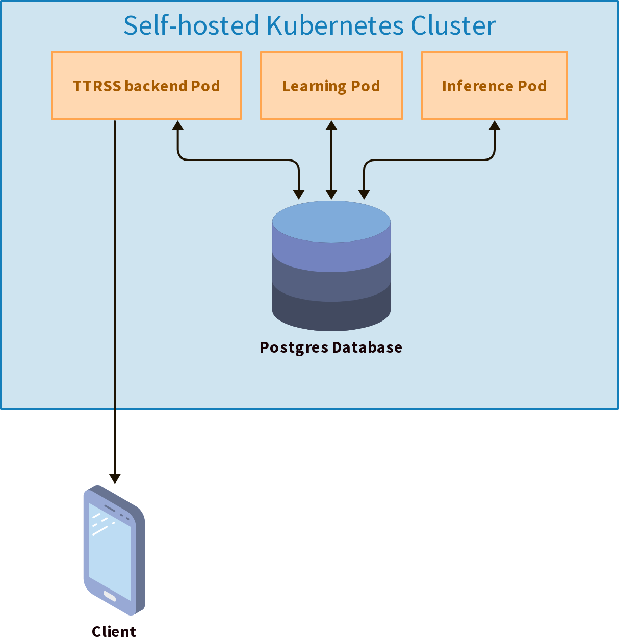
The architecture for this project is pretty straightforward. I will deploy two new pods onto my Kubernetes cluster:
- A learning pod: this pod will be responsible for training the relevance model (a binary classifier). It will access the database to get the articles and their classification (liked/disliked), and fine-tune a ModernBERT model on this data
- An inference pod: this pod will be responsible for scoring the
articles. It will access the database to get the articles and use two
models to score them:
- the fine-tuned ModernBERT model (created by the learning pod) to predict the relevance of each article
- a quantized Ministal 8B instruct model to predict the time sensitivity of each article (how quickly an article becomes irrelevant)
This is made very simple by the fact that I own the PosgreSQL database. The pods can go straight to the source and read/write directly to the database.
Articles data
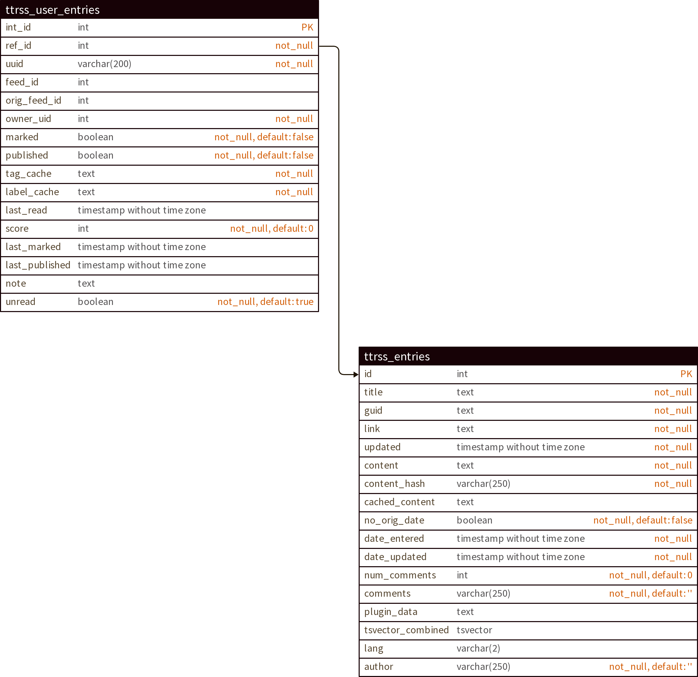
TTRSS creates multiple tables in the database. The two most important ones are:
ttrss_entries: contains all the articles, with their title, content, URL, author, publication date, etcttrss_user_entries: contains the user-specific data for each article, such as whether the article has been read, liked, a user-assigned score, etc.
To train our binary classifier, we will look at the articles that the user
labelled: an article is considered labelled if the user read it (unread is
false in ttrss_user_entries), or if the user published it (published is
true in ttrss_user_entries). A read article is a POSITIVE example (the
user was interested in the article), a published article is a NEGATIVE
example (the user was not interested in this article).
NOTE: the published field is not meant to be used this way. In TTRSS,
users can click on the “publish” button for an article to add the article to
their own RSS feed. They can share the URL of their own feed with followers
to “relay” to others which articles they find interesting. I don’t use
this feature, so I hijacked the “published” button to label articles as
uninteresting. This is because the “publish” button is conveniently placed
and allows me to quickly mark articles as uninteresting:

Finally, TTRSS is meant to be a multi-user application, so the data in
ttrss_user_entries is linked to a specific user through the owner_uid
field. But in my case, I am the only user of this TTRSS instance, so I
ignored this field.
Training a relevance classifier
Choosing the right model
My goal was to estimate the relevance of any new, unread article that TTRSS collects from any site/blog that I follow. This can be done with a textbook implementation of a binary classifier:
- The classifier is trained on two classes:
POSITIVE(interesting article) andNEGATIVE(uninteresting article). For that, it needs labelled positive and negative examples - Once trained, the classifier is presented with an unknown (unread) article
for inference. The classifier outputs some sort of probabilities for the
article to belong to the positive and negative classes,
P(POSITIVE)andP(NEGATIVE). To simplify, let’s say thatP(POSITIVE) + P(NEGATIVE) = 1. We can then useP(POSITIVE) * 100as the relevance score, which ranges from 0 to 100
Training a binary classifier for this kind of task is actually a very common approach (when you have labelled data); so common that Hugging Face has a recipe about it. It perfectly fitted my situation, since I already had some labelled data.
If we look at it in details, the model I will be using (a model from the BERT family) is an encoder-only model. More details about models’ architecture can be found here, but in a nutshell, encoder-only models are best suited for tasks requiring an understanding of the full sentence, such as sentence classification. This property is due to how this class of models is trained: during their training, encoders have access to the whole sentence, and the training task usually revolves around somehow corrupting a given sentence (for instance, by masking random words in it) and asking the model to find or reconstruct the initial sentence. By contrast, decoder models are trained only of the previous words in a sentence, and are asked to predict the next word. These days, modern LLMs (like the ones used by ChatGPT) are decoder-only models.
Encoder and decoder models each have their use, but encoder models tend to be much smaller than decoder models. That makes them cheaper and faster to train, and cheaper and faster for inference. If properly fine-tuned for a task, encoder models often outperform decoder models.
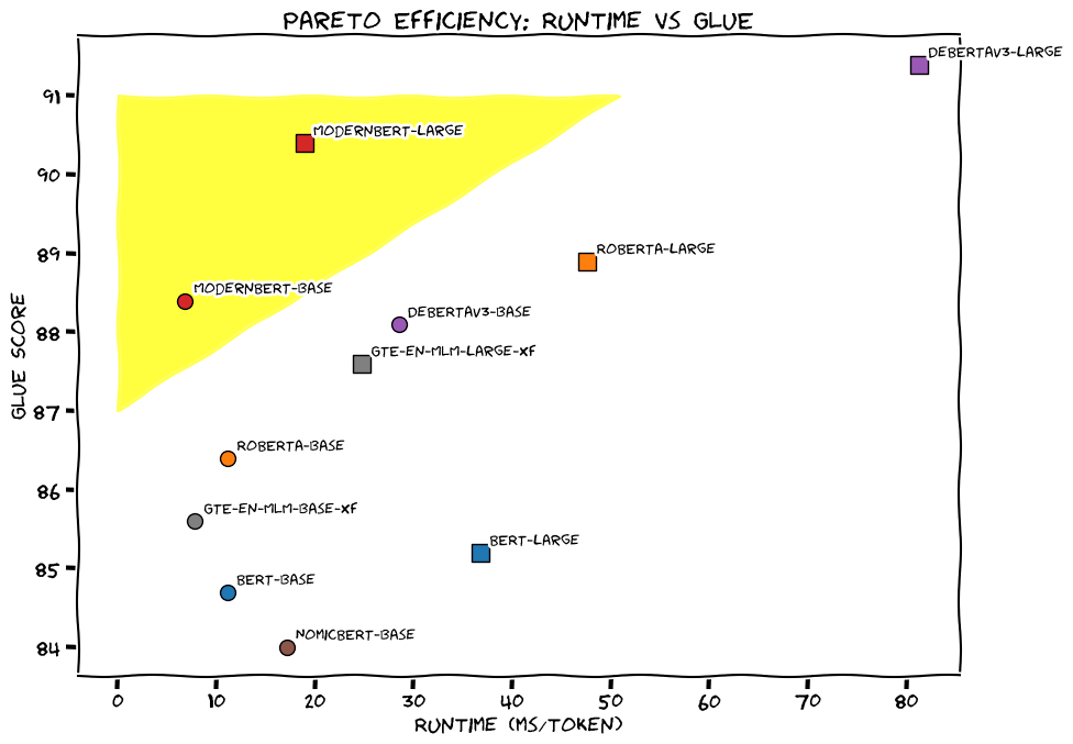
I decided to follow Hugging face’s recipe for text classification, but I opted to use ModernBERT base, a drop-in replacement for the DistilBERT model used in the recipe. According to this blog post, ModernBERT is an improvement over the previous generations of BERT:
Training the model
Actually training the model was easier than I thought it would be, thanks to Hugging face’s libraries. The full code for training the relevance model is available here. I will explain my approach through the following sections.
Pulling the training data
I decided to pull all the read (POSITIVE) and published (NEGATIVE) articles from the past year. One year seemed a good enough threshold; I have older data than that, but my interests probably changed over time, and I wanted the model to learn only my most recent interests. This gave me approximately 2360 positive articles, and 620 negative articles. This is an unbalanced dataset, so I truncated the number of positive articles to 620 articles. Finally, I isolated 100 positive and 100 negative articles for the evaluation of the model. The content of the articles was then sanitized (for example, html tags were stripped).
Fine-tuning the model and model output
Once I figured out what data to use for the training step, actually fine-tuning the model was easy. I experimented with a few things, in particular the number of epochs (how long the model is trained on the data) and what metric to use during the training:
- I found that using more than 2 epochs did not yield any better results. It just takes more time to train the model
- I ended up using the “average precision” metric for the training, because it rewards the model for ordering things correctly so that the real positives appear earlier than the false ones (since ranking articles by relevance is my actual goal)
Fine-tuning the model with this amount of data (roughly 1000 articles) takes around 3 minutes with my GPU (RTX 3060), and around 30 minutes on my CPU. That’s the beauty of encoder-only models: they can be trained to do useful things in a reasonable amount of time, even on CPUs.
To output a relevance score during inference, I decided to use a sigmoid
function over the logit for the positive class that the model outputs for
any given article, multiplied by 100. This doesn’t give P(POSITIVE)
strictly speaking (since the probabilities are not calibrated), but it
gives a score totally usable for ranking the articles among each other.
Evaluation
Once the model was trained, I evaluated its performance against a validation set of 100 positive articles and 100 negative articles. These are the performance metrics I obtained:
Precision: 0.91
Recall: 0.87
F1 score: 0.89
ROC AUC: 0.95
Average Precision: 0.92
- Precision (0.91): Of all the instances the model predicted as positive, 91% were actually positive
- Recall (0.87): The model correctly identified 87% actual positive instances (13% false negatives)
- F1 score (0.89): The harmonic mean of precision and recall, balancing both into a single score
- ROC AUC (0.95): The probability that the model ranks a randomly chosen positive higher than a randomly chosen negative
- Average Precision (0.98): The area under the precision–recall curve, summarizing precision across different recall levels
These are pretty solid metrics!
Training a time sensitivity classifier
Time sensitivity is one aspect of news-surveying that I always found difficult to tackle: some pieces of news are relevant forever, while some other are only relevant for a couple of days. Some news expire faster than others. For example, a commentary of Jean-Paul Sartre’s autobiography will be relevant forever, while the end of a war between two countries will be relevant only a couple of days (not that it wouldn’t be important anymore after that, but I would have heard about it through another channel than my RSS feeds). To me, each news has an intrinsic time sensitivity that doesn’t change over time. I came up with five categories of time sensitivity:
- 1 (Evergreen): Content is historical, biographical, or a foundational explainer
- 2 (Low): A feature, trend analysis, or opinion piece relevant for months
- 3 (Medium): Story tied to an ongoing but not breaking event, relevant for days/weeks
- 4 (High): Reports on a specific, recent event; loses relevance in 24-48 hours
- 5 (Critical): Live coverage of a rapidly unfolding event; loses relevance in hours
Exponential decay of relevance over time
My initial idea was simple: if I can assign a time sensitivity score to an article, I can adjust the relevance of this article over time with a simple exponential decay:
R(t) = R0 · e-kt
Where:
- R(t) = The relevance score at a specific time t
- R0 = The initial relevance score, output of the previous binary classifier
- k = The decay constant, which I’ll set based on the time-sensitivity score
- t = The time elapsed since publication (e.g., in days).
- e = Euler’s number (approximately 2.718).
The decay constant is a half-life constant, which is set for every time sensitivity score. It’s computed like this:
k = ln(2) / t1/2
For example, let’s assume that an article with a time sensitivity of 4 will lose half of its relevance in two days:
k = 0.693 / 2 = 0.35
If the article has an initial relevance of 85, we can compute its relevance at two days:
R(2) = 85 · e-0.35 · 2 = 42
Two days after its publication, the article’s score will be 42, compared to 82 when it was published. This makes sense (at least to me): if an article expires quickly, it will be relevant only for a short amount of time. Since its score decreases over time, this article will not be at the top of my list when I sort the articles by score. Other articles can take its place at the top of the list.
Assigning a time sensitivity score
Unfortunately, I don’t have labelled data when it comes to time sensitivity. If I had, I could theoretically train an encoder model on it. I could use the same approach as before, but with five classes instead of two. For this particular problem, I used an decoder-only model: Ministral 8B Instruct, or more precisely, a quantized version of Ministral 8B instruct. My GPU only has 12GB of VRAM, and the original model would not fit into memory. I used the Q6 quantization, and the model takes around 6.5 GB of VRAM once loaded.
This model works differently than ModernBERT. It’s a decoder model and it’s much bigger: 8 billion for Ministral, 150 million for ModernBERT. I didn’t fine-tune the Ministral model (not a chance with my GPU), I used it as is and prompted it instead. This kind of models is called instruct because they’re trained to follow instructions. Here is the prompt I’m using:
[INST]
You are a news analysis AI that evaluates the time-sensitivity of news articles.
Your sole function is to return a valid JSON object based on the provided data.

**Objective:**
Analyze the provided article information and determine its time-sensitivity rating on a scale of 1 to 5.
Time-sensitivity refers to how quickly the information becomes outdated, not its overall importance.

**JSON Output Schema:**
{
  "score": <integer between 1 and 5>,
  "confidence": <string, "high", "medium", or "low">,
  "explanation": <string, a concise explanation for the rating>,
}

**Rating Scale Definitions:**
- **1 (Evergreen):** Content is historical, biographical, or a foundational explainer.
    Keywords: "history of", "profile", "explainer", "deep dive".

- **2 (Low):** A feature, trend analysis, or opinion piece relevant for months.
    Keywords: "analysis", "opinion", "trend", "culture".

- **3 (Medium):** Story tied to an ongoing but not breaking event, relevant for days/weeks.
    Keywords: "debate", "upcoming", "policy", "investigation".

- **4 (High):** Reports on a specific, recent event; loses relevance in 24-48 hours.
    Keywords: "announces", "reports", "wins", "results", "verdict".

- **5 (Critical):** Live coverage of a rapidly unfolding event; loses relevance in hours.
    Keywords: "live", "breaking", "unfolding", "evacuation", "alert".

**Instructions:**
Analyze the following article. Provide your response as a single, valid JSON object and nothing else.
Do not include any additional text, labels, or markdown formatting.
Ensure your JSON is well-formed and valid.

**Article Data:**
Title: <headline>
Summary: <article_summary_or_first_paragraph>
[/INST]
In the prompt, I’m telling the model:
- To act as a news analysis AI
- To output a response in the JSON format. I specify the schema of the response
- To choose among the five time sensitivity categories. I provide guidelines for choosing
There are two placeholders at the end of the prompt: <headline> and
<article_summary_or_first_paragraph>. During inference, these placeholders
are replaced - for each article - by the article title and the article
content. And for each article, the model outputs a JSON object containing
the time sensitivity score, a confidence level, and an explanation that
justifies the score (not strictly necessary, but I use the explanation to
assess the performance of the model).
Inference with Ministral is not fast: around 1.4 second per article (I could probably shorten that by getting rid of the explanation and the confidence level). However, each article only needs to be assessed once with this model. I store the time sensitivity scores in the database, in a table I created specifically for this:
create type confidence as enum (
    'low',
    'medium',
    'high'
);

create table time_sensitivity (
    article_id integer primary key references ttrss_entries(id) on delete cascade,
    score integer not null default 0,
    last_updated timestamp with time zone not null default now(),
    confidence confidence,
    explanation text
);
Also, I could potentially use the time sensitivity scores generated by Ministral as labelled data to train an encoder model…
Putting everything together
I have two models:
- A fine-tuned ModernBERT binary classifier, that outputs a relevance score for every article
- A prompted Ministral model, that outputs a time sensitivity score for every article
As described in the “Exponential decay” section, I can use the relevance score, the publication date and the time sensitivity score to continuously score my RSS articles. Over time, older articles will be superseded by more fresh/relevant articles.
The final inference script is here. I run the inference script every 30 min. Every 30 minutes, the Ministral model assesses the time sensitivity of all new articles since the previous run. Then, the trained ModernBERT model provides a relevance score for all the unread articles of the past 30 days. The relevance and time sensitivity scores are used in conjunction with the publication date of every article to finally output a time-adjusted relevance score.
Effectively, the unread articles of the past 30 days are re-scored every 30 minutes (but the time sensitivity of each article is only assessed once, since this is an expensive operation). This is because the overall relevance score is affected by time passing.
Since some of the half-lives I use are larger than 30 days, I also randomly re-score some articles that are older than 30 days, but more recent than 1 year. But not all the articles in this range are re-scored every 30 minutes, only a fraction of them, to save on compute time.
DECAY_RATES = {
    1: 0.0019,  # Half-life of 365 days
    2: 0.004,  # Half-life of 183 days
    3: 0.0231,  # Half-life of 30 days
    4: 0.069,  # Half-life of 10 days
    5: 0.139,  # Half-life of 5 days
}
The relevance classifier training script is run every day at 1 am. Since I use the app everyday, I label more data every time I use the app, and the amount of training data continuously increases. Continuous training keeps the relevance classifier in sync with my interests.
Conclusion
Below is a screenshot of how the Android app looks like when it shows scored articles. I voluntarily decided to prefix the titles with the time-adjusted relevances, and to suffix them with the time sensitivities. This wasn’t necessary because the final scores are stored in the database and the app can sort based on score, but it allows me to quickly see what’s happening under the hood.
As of 31/08/2025, the relevance classifier has been running for a few weeks, and the time sensitivity one has been running for a few days. I am absolutely astonished by the quality of the recommendations. When I sort by score, the unread articles at the top of the list are all interesting. I thought that the relevance classifier alone was already amazing, but the time sensitivity classifier helped with clearing the top of the list from high time sensitivity articles that stayed there for too long.
I will keep monitoring the quality of the ranking, and I might adjust the decay constants, but I’m already extremely satisfied with the results.